
In my previous blog post, No pie charts – The basics of visual perception, I ranted about the poor visual perception of pie charts and had examples about better ways of give the reader insight. This post will try to give an overview of all charts and diagrams I find useful, dependent of the data.
A good overview of supported charts for different libraries and tools can be found at The chartmaker directory. In this post, I will only look at a subset of the charts presented there, but will in later posts come back to how we can use specialized and customized charts to see how this can provide more insight to data. Often, this is accompanied with calculations before presentation. And, we can also combine several charts into a dashboard, and use the presentation medium to our advantage. Now, we concentrate on the basics…let’s go!
Time series
Personally, I find time series very interesting. They are a natural part of our daily life, and even though they are simple, they contain much information. We will distinguish between univariate and multivariate series. For simplicity, we can say that a univariate series will have a time component and one corresponding value, whilst a multivariate can have several variables at the same time. Multivariate is a big research field when it comes to analysis and statistics.
Observations at points
When you have observations that are recorded along with their time stamps, then generally the choice of chart should be a line chart. Time should be along the x-axis, from left to right, and values should be along the y-axis.
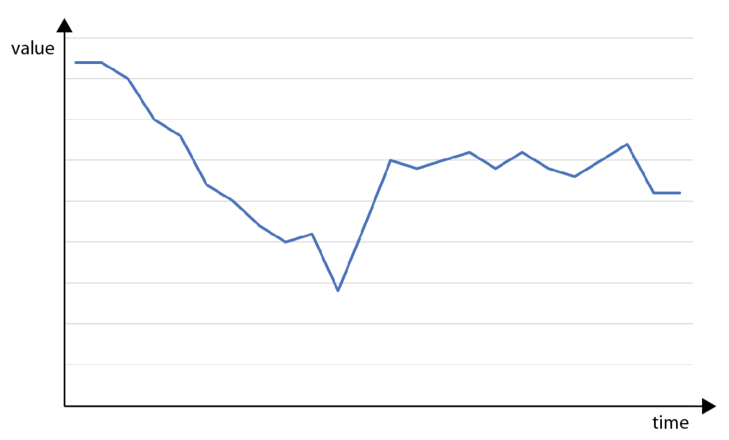
Time series in a generic line chart
If the you want a smoother chart between points, then many libraries let you chose spline. Spline will interpolate a polynomial between the points so it seems like the observation were continuous.
Time axis
The example chart above has no values on the time axis. Having values shown on the y-axis is easy, as you can just put them there more or less, but a point in time can consist of date and time information which should be formatted correctly. Consider the following chart:
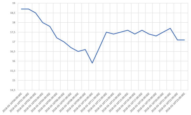
Time series – with UTC time stamps
This chart will not be visually pleasing as the time labels are too long and too many. We can remove half of them and show only the time component without confusing the reader, like this:
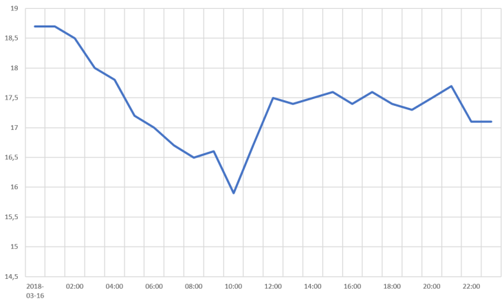
Time series – formatted time stamps
Have look at both charts and see where it’s easiest to spot the time of the minimum value!
There are also some general rules I apply to time axis considering the resolution of the data. When we have values that are calculated over a period and then want to record that calculation, it will be mathematically correct to set the timestamp at the end of the period. E.g. if I want the average of the values above, over a day, I will get 17.4 at 2018-03-17T00:00:00. Notice that this time stamp actually is the next day. It’s not 23:59:59 or something even closer to midnight, but a time stamp of 00:00:00 indicates up to, but not including, midnight when we have a calculation like ours. However, when showing this value in a chart, that value should appear without a time component, and for the day 2018-03-16. Using a column chart may be a better choice in some cases, e.g. if we say that the values in our chart was the hourly averages, then we could visualize this as:

Column chart
Another detail to consider is time stamps with time zone offset. In order to synchronize time stamps, they should be recorded as UTC or with the time zone offset. When presenting those data to the user, one must take into account what the user expects in terms of time zone information. Most users will not care and expect data to be shown with same time zone as they originated, but this can differ. Companies with branches in different time zones will face this challenge e.g. when looking at sales on Monday. Then they probably will have local Monday for each branch. Additional challenges can arise when we have daylight savings switching, where a day suddenly gets 25 or 23 hours.
Augmenting the chart
By augmenting the chart, I mean adding additional information to the chart that will give the user addition insight in e.g. what chart properties like maximums and minimums represent. It’s common to have a threshold band in which the data values are supposed to be, but one can also add a number of KPIs.
If we look at our data set, the negative trend that had a minimum and then seemed to stabilize at a somewhat middle value, could be explained by adding information as shown in the chart below:

Augmented chart
The skilled reader will now see that somebody did maintenance on something that the data set represents. After this, the efficiency dropped to a minimum, where an alarm was triggered and a corrective action performed, and then the efficiency was measured to be in a band indicated as the optimized.
More than one line in the same chart
When we have data sets with same time stamps, or there’s a need for comparing two or more separate data sets by shifting the time stamps to some periodicity, then we can add more lines to our chart. One thing to consider here is proper use of colors, as color often is used to distinguish between the data sets. Tools like ColorBrewer can be very valuable in these cases. Multiple lines would require some kind of legend to explain the color coding, as shown in the following chart:
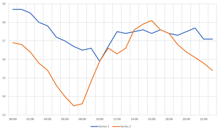
Line chart – multiple data sets
The limitation for how many lines to show depends. If you want to show each line in a separate color, then stop at 4-5. If you want to highlight one line together with a huge number of others, make that line in a color and the rest in a common gray or similar. The latter will give the user a good sense of how the highlighted data set is compared to the spread of the rest. Which brings us into the question: Why do you want to show a huge number of charts? Are there any special pattern you try to see, like last value, minimums or maximums, trends or outliers? If so, then consider other visualizations where those points of interest are compared.
Multiple charts for comparisons
Instead of having all data sets plotted in one chart, there’s also the option to use multiple charts. When the intention is still to compare values, the one important thing is to use the same value range for all y-axis. The following example shows how difficult it is to compare Series 4 with the rest since the y-axis differs:

Multiple time series – Not same value range on y-axis
Trending and forecasting
One of the main reason for using a line chart for time series will be because time series represents development over time. Humans will then have a natural way of see trending and forecast future values. The two most useful trends to be plotted along the time series will be a linear or exponential, but this depends on the nature of the data and what pattern to expect.
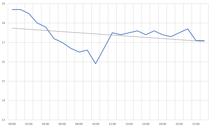
Time series – with a linear trend line
When not to use a line chart for time series
In many cases, time is not the important component. Probably in more cases that we believe, as the line chart with time on the x-axis is the go-to chart for most people. As for all (useful) charts, they are just there to make it easier to gain insight. As I’ve said previously, if you e.g. are after maximum values, then present this as a number (and time) instead. Instead of plotting several data sets in one or more charts for comparison, then plot the maximum in bar charts. And similarly with other properties.
Another case could be data sets along geographical coordinates. Typically, then a map is used, and it will make more sense to have distance instead of time for showing what happened at certain points, like my chart from Strava for a bike trip shows:
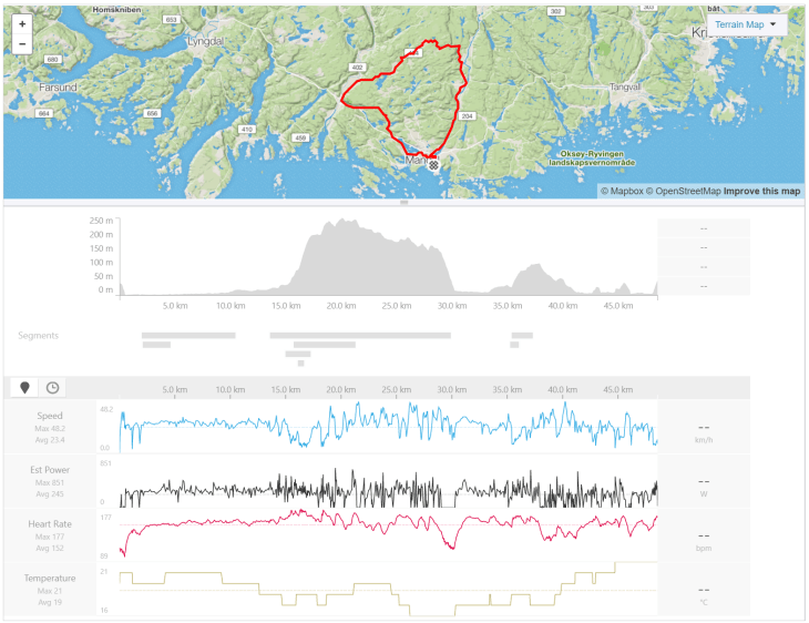
Charts from Strava
Comparing quantitative data
In many cases, a simple bar or column chart will do the job when we want to compare quantitative data. This was also shown in No pie charts – The basics of visual perception.
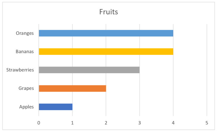
Bar chart
It’s also easy to add additional information to the bar chart, like targets.
Patterns in quantitative data
When there are patterns in the data that should be compared across different categorical values, we have the option of using multiple charts or have multiple elements for each category in one chart. Both can end up with hard to read charts. Another chart that can be useful in these cases are heat maps.
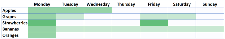
Simple heatmap
Let’s say we try to understand more about the quantities for our fruits in the example above. We now want to see if we can spot any patterns, say, for the days of the week. When we plot the values in an heat map where the color indicate a quantitative value, we can draw some conclusions, like
- Mondays are the best for all fruits
- Apples are best early in the week
- Grapes seems to have good days followed by two bad
- Strawberries have the highest number, but only for two days
- Bananas don’t depend so much on days
- Oranges are for Mondays
- Thursdays and Sundays are the two worst days in the week
The next thing from this chart is to take some action. Maybe I want to examine closer why strawberries peak at Mondays and Fridays, maybe we go out of stock on Monday and have to wait until Friday to get fresh ones, maybe we can price them higher at the days with most demand, etc.
Finding correlations in data sets
In cases where two data sets should correlate, a scatter plot may reveal the relations. The chart below takes one point from each data set and mark this with a circle. The plot clearly shows a linear correlation between the sets as all points lie on a straight line.
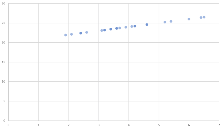
Scatter plot with correlation in data sets
A famous set of data is Anscombe’s quartet. The numbers in these sets don’t give the reader any easy insight, but scatter plots make this obvious.
To sum up
This ended to be a long post about time series, and not so much about the rest of charts that exist. However, the charts presented here really make up some of the basis for data visualization, and they can provide good insights to the data they represent. Often, the real challenge is not to find the correct chart, but to examine and transform the data according to what question that should be answered.
